Initial value problems calculus worksheet

We look at techniques for integrating a large variety of functions involving products, quotients, and compositions later in the text. Here we turn to one common use for antiderivatives that arises often in many applications: solving differential equations.

A differential equation is an equation that relates an unknown function and one or more of its derivatives. The equation

is a simple example of a differential equation. Solving this equation means finding a function [latex]y[/latex] with a derivative [latex]f[/latex]. Therefore, the solutions of [latex]\frac[/latex] are the antiderivatives of [latex]f[/latex]. If [latex]F[/latex] is one antiderivative of [latex]f[/latex], every function of the form [latex]y=F(x)+C[/latex] is a solution of that differential equation. For example, the solutions of

Sometimes we are interested in determining whether a particular solution curve passes through a certain point [latex](x_0,y_0)[/latex]—that is, [latex]y(x_0)=y_0[/latex]. The problem of finding a function [latex]y[/latex] that satisfies a differential equation

with the additional condition

is an example of an initial-value problem. The condition [latex]y(x_0)=y_0[/latex] is known as an initial condition. For example, looking for a function [latex]y[/latex] that satisfies the differential equation

and the initial condition

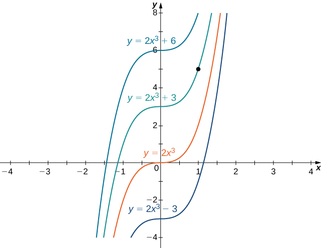
is an example of an initial-value problem. Since the solutions of the differential equation are [latex]y=2x^3+C[/latex], to find a function [latex]y[/latex] that also satisfies the initial condition, we need to find [latex]C[/latex] such that [latex]y(1)=2(1)^3+C=5[/latex]. From this equation, we see that [latex]C=3[/latex], and we conclude that [latex]y=2x^3+3[/latex] is the solution of this initial-value problem as shown in the following graph.

Figure 2. Some of the solution curves of the differential equation [latex]\frac=6x^2[/latex] are displayed. The function [latex]y=2x^3+3[/latex] satisfies the differential equation and the initial condition [latex]y(1)=5[/latex].

Example: Solving an Initial-Value Problem

Solve the initial-value problem

First we need to solve the differential equation. If [latex]\frac= \sin x,[/latex] then

Next we need to look for a solution [latex]y[/latex] that satisfies the initial condition. The initial condition [latex]y(0)=5[/latex] means we need a constant [latex]C[/latex] such that [latex]− \cos x+C=5[/latex]. Therefore,

The solution of the initial-value problem is [latex]y=− \cos x+6[/latex].

Try It

Solve the initial value problem [latex]\frac=3x^, \,\,\, y(1)=2[/latex].

Find all antiderivatives of [latex]f(x)=3x^[/latex].

Watch the following video to see the worked solution to Example: Solving an Initial-Value Problem and the above Try It.

For closed captioning, open the video on its original page by clicking the Youtube logo in the lower right-hand corner of the video display. In YouTube, the video will begin at the same starting point as this clip, but will continue playing until the very end.

Try It

Initial-value problems arise in many applications. Next we consider a problem in which a driver applies the brakes in a car. We are interested in how long it takes for the car to stop. Recall that the velocity function [latex]v(t)[/latex] is the derivative of a position function [latex]s(t)[/latex], and the acceleration [latex]a(t)[/latex] is the derivative of the velocity function. In earlier examples in the text, we could calculate the velocity from the position and then compute the acceleration from the velocity. In the next example, we work the other way around. Given an acceleration function, we calculate the velocity function. We then use the velocity function to determine the position function.

Example: Decelerating Car

A car is traveling at the rate of [latex]88[/latex] ft/sec ([latex]60[/latex] mph) when the brakes are applied. The car begins decelerating at a constant rate of [latex]15[/latex] ft/sec 2 .

1. How many seconds elapse before the car stops?
2. How far does the car travel during that time?

1. First we introduce variables for this problem. Let [latex]t[/latex] be the time (in seconds) after the brakes are first applied. Let [latex]a(t)[/latex] be the acceleration of the car (in feet per seconds squared) at time [latex]t[/latex]. Let [latex]v(t)[/latex] be the velocity of the car (in feet per second) at time [latex]t[/latex]. Let [latex]s(t)[/latex] be the car’s position (in feet) beyond the point where the brakes are applied at time [latex]t[/latex].
   The car is traveling at a rate of 88 ft/sec. Therefore, the initial velocity is [latex]v(0)=88[/latex] ft/sec. Since the car is decelerating, the acceleration is